One Sunday morning, I was attempting to irritate my older brother by asking him questions about his job. He is an IT professional, so I asked him if he used Microsoft Excel often. With an unimpressed tone he replied, “Who still uses Excel?”
I wondered what type of Twilight Zone universe he was living in because I use Excel everyday – it is an absolute necessity in both my professional and personal life.
In fact, I’ve heard the joke a few times that Microsoft Excel is akin to the Greek god Atlas.

Since I belong to the finance world, I always thought it important to understand how to leverage this powerful tool to make more efficient financial models.
In my quest to harness a high level of efficiency in my models, there are a few functions that are quite useful in creating a dynamic model but may not be that popular.
I’ve picked three functions to focus on for the rest of the article. We will explore in detail how each function is used with examples:
- TEXTJOIN
- INDIRECT
- INDEX AND MATCH
TEXTJOIN
The TEXTJOIN function combines text from multiple ranges into a single string.
TEXTJOIN (delimiter, ignore_empty, text1, [text2], …)
The TEXTJOIN function has the following arguments:
- Delimiter: a required field that specifies the separator to be inserted between each entry. Common delimiters are commas, blank spaces and semi-colons
- Ignore_empty: a required field in which the user must select “TRUE” to ignore empty cells or “FALSE” to do the opposite
- Text1, Text2,…,TextN: the entry/ text to be joined into one string
The following examples are accompanied by screenshots.
Example 1:
Suppose we have five stocks each belonging to a different industry with a unique beta.
Task: We want to list all the investment securities in a single cell.
Execution: In the formula, type the following parameters –
- The delimiter “,”
- Type “True” or “1” to ignore empty cells
- The range: “$A$2:$A$6”
The formula is shown in cell F3 below.
There are many ways to perform this simple task in Excel such as using CONCAT or a basic formula with the ampersand (=text1&”, “&text2…). However, TEXTJOIN makes life easier by allowing the user to state the delimiter upfront and account for empty cells.

INDIRECT
The INDIRECT function is used to obtain a value from a cell using the cell reference. The cell reference is entered as a text string.
INDIRECT(ref_text, [a1])
The INDIRECT function has the following arguments:
- Ref_text: a required field in which the cell reference/range is entered as a text string, for example, “C1”
- A1: an optional field which specifies the type of reference used for the ref_text. If TRUE or omitted the ref_text will be classified as an A1 cell reference – column label is followed by row label. If FALSE, the ref_text will be classified as an R1C1 cell reference – row label is followed by column label
Example 2:
Building on Example 1 suppose we want to return the beta value for a particular stock.
Task: Return the beta value for Stock A in cell F4.
Execution: In the formula type “C2” for the ref_text field.
The formula is shown in cell F5.
The indirect formula converts the text string “C2” into the cell value contained in cell C2. This is used instead of directly referencing the cell by typing “=C2” in cell F4. While this simple example may not seem practical, for more complex computations it allows the user to create dynamic ranges.

Example 3:
Suppose we have three bond portfolios and the respective face values of bonds held in each sector.
Task: We want to calculate the total face value for each portfolio.
Execution: For each portfolio, name the face value ranges: Portfolio_1, Portfolio_2 and Portfolio_3 respectively. Nest the indirect formula within the sum formula.
In the indirect formula type “$F$3” for the ref_text field. In G3, we can see the total face value for Portfolio 1. If the user wants the total face value for the other portfolios, they will only have to change the reference name in cell F3. No changes are made to the formula itself, which is great if you want dynamic calculations.

INDEX AND MATCH
As the name suggest, Index and Match is a combination of two functions index() and match(). It is a dynamic lookup function which does not rely on the user to manually enter column references like the VLOOKUP function.
We will look at the component parts of INDEX and MATCH.
INDEX(array, row_num, [column_num])
The INDEX function has the following arguments:
- Array: a required field that specifies a range of cells
- Row_num: required if the column_num is not specified. It returns a value from the row specified within the range
- Column_num: an optional field which returns a value from the column specified within the range. If omitted the row_num is required
Example 4:
Task: Using the same table from Example 1 and 2, suppose we want to return the beta value for Stock C using the index formula.
Execution: In the formula, type the following parameters –
- Array: $A$1:$C$6
- Row_Num: 4
- Column_Num: 3
The index formula returns the value in the 4th row and 3rd column within the specified array. This returns the beta value for Stock C. See formula in cell F8.

Instead of manually entering the row and column numbers the MATCH formula can return a specific location in a range of cells.
MATCH(lookup_value, lookup_array, [match_type])
The MATCH function has the following arguments:
- lookup_value: a required field that specifies the value you want to match in the range
- lookup_array: a required field that specifies a range of cells
- match_type: an optional field where the user can specify to return an exact match (0) or non-exact match (1,-1)
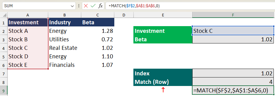
Execution: In the formula type, the following parameters –
- Lookup_value: $F$2
- Lookup_array: $A$1:$C$6
- Match_type: 0
The formula returns the row number in which “Stock C” is located – row 4.

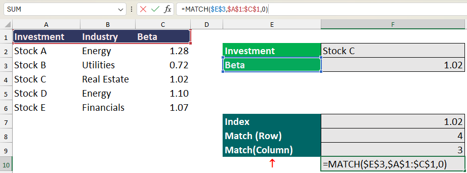
The match formula is also used to return the column number as seen below.

Finally, the index and match formula can be completed by including both match functions in the index formula as seen in Example 4.
Below shows the complete formula:
Instead of manually entering the row and column numbers, the match formula does the heavy lifting for you.

This brings us to the end of the article. I hope it was insightful and if you know any other interesting Excel functions, please feel free to share them in the comment section below!
The template below contains the examples used in this article. A practice and answer sheet is provided for each example.
